Example session

Let us start with an example of using the fern plugin. You will see how to load a fernml network, how to simulate it and visualize the progress and how to produce trend curves of some species.

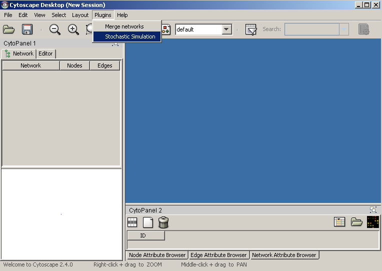
Start cytoscape and activate the plugin.

Figure: Cytoscape plugin example - step 1

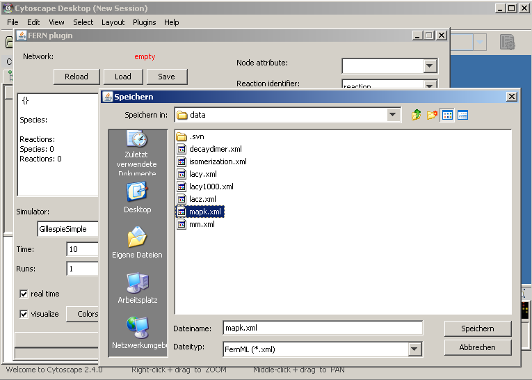
Click the load button in the upper left corner of the plugin window and choose a fernml file from your filesystem (there are some examples included in the fern package - let us use mapk.xml).

Figure: Cytoscape plugin example - step 2

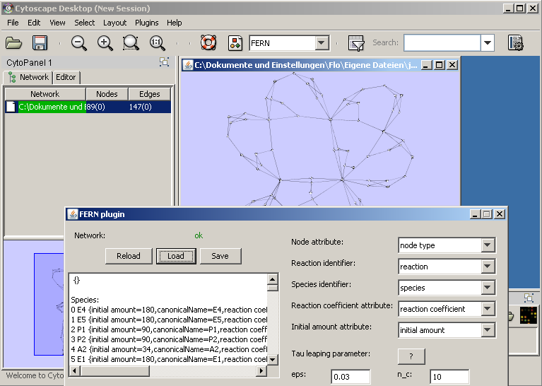
Now we can see that the network is loaded correctly, but since fernml does not specify a graph layout, let us beautify the view and pick an automatic layout (e.g. the organic one from the yFiles plugin).

Figure: Cytoscape plugin example - step 3

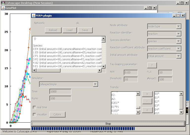
Since the interesting dynamics of this network emerge during a time period of 1000 units [1], we change this value. Now we can start the simulation with everything else set to default (don't forget to look at the cytoscape main window!).

Figure: Cytoscape plugin example - step 4

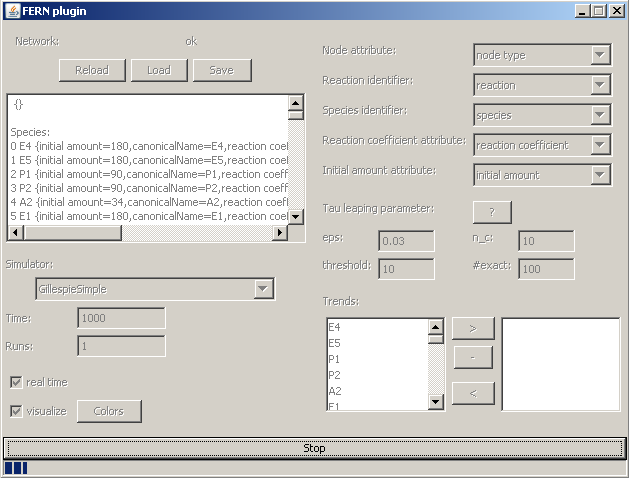
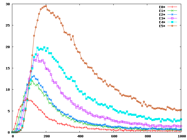
Because we had real time checked, the simulation will last at least 1000 seconds. Because we don't want to wait so long, we stop the simulation. Now let us produce some nice trend curves. Uncheck real time and visualize and move the E0* to E5* to the right of the two lists in the lower right corner. We want an average trend of 100 runs, so we fill in that value. Now we can restart the simulation.

Figure: Cytoscape plugin example - step 5

If you want to save the plot, you simply have to click onto it.

Figure: Cytoscape plugin example - step 6